Physics enforced
operator learning.

Nematic elastomers are rubber-like polymer networks coupled to an orientational order, so the deformation and the director field must be found together. This is the setting of the paper below, which formulates the problem for microstructured media and develops neural network and operator-learning solvers whose output is checked against necessary stability conditions^[1]. The material is described by the following theory.

Operator learning, and how it is validated

GeometryBoundary conditionsMaterialLoading

↓

Neural operatorDeepONet · FNO

↓

Physical fieldsdeformation · director · temperature · concentration

↓

Validation against FEAnode by node against FEM / NEM · stability checks

Conceptual formulation. In this project the operator input is the load level; geometry and material as inputs are the goal. The numbers above are for the 156-node plane-strain benchmark.

The problem: Cosserat elasticity with a unit director

The material is modeled as a Cosserat continuum with a single unit director. Two kinematic fields describe the body: the deformation \( \boldsymbol{x}=\boldsymbol{\chi}(\boldsymbol{X}) \) and the director \( \boldsymbol{d}(\boldsymbol{X}) \), subject to the constraint \( \boldsymbol{d}\cdot\boldsymbol{d}=1 \). The stored energy per unit reference volume depends on both fields and on the director gradient,

Frame invariance requires \( W(\boldsymbol{F},\boldsymbol{d},\nabla\boldsymbol{d})=W(\boldsymbol{Q}\boldsymbol{F},\boldsymbol{Q}\boldsymbol{d},\boldsymbol{Q}\nabla\boldsymbol{d}) \) for every rotation \( \boldsymbol{Q} \). With the generalized stresses \( \boldsymbol{P}=\partial W/\partial\boldsymbol{F} \), \( \boldsymbol{N}=\partial W/\partial\boldsymbol{d} \) and couple stress \( \boldsymbol{M}=\partial W/\partial\nabla\boldsymbol{d} \), this is equivalent to

Equilibrium is a stationary point of the total potential energy \( \mathcal{E}=\int W\,dV-\mathcal{L} \). Varying \( \boldsymbol{\chi} \) freely and \( \boldsymbol{d} \) subject to \( \boldsymbol{d}\cdot\delta\boldsymbol{d}=0 \) gives the balance of linear momentum and of director momentum,

with \( \boldsymbol{f},\boldsymbol{l} \) the body force and body couple. A network trained on \( \mathcal{E} \) is driven toward such a stationary point.

Constitutive model

For the planar simulations shown below, the energy is of neo-Hookean type with an anisotropic network metric, plus a Frank-type director-gradient term:

where \( \boldsymbol{D} \) is the initial director, \( \mu \) the shear modulus, \( \alpha \) the Frank modulus and \( \gamma \) a size-effect length. The corresponding stresses and couples are

Simulations

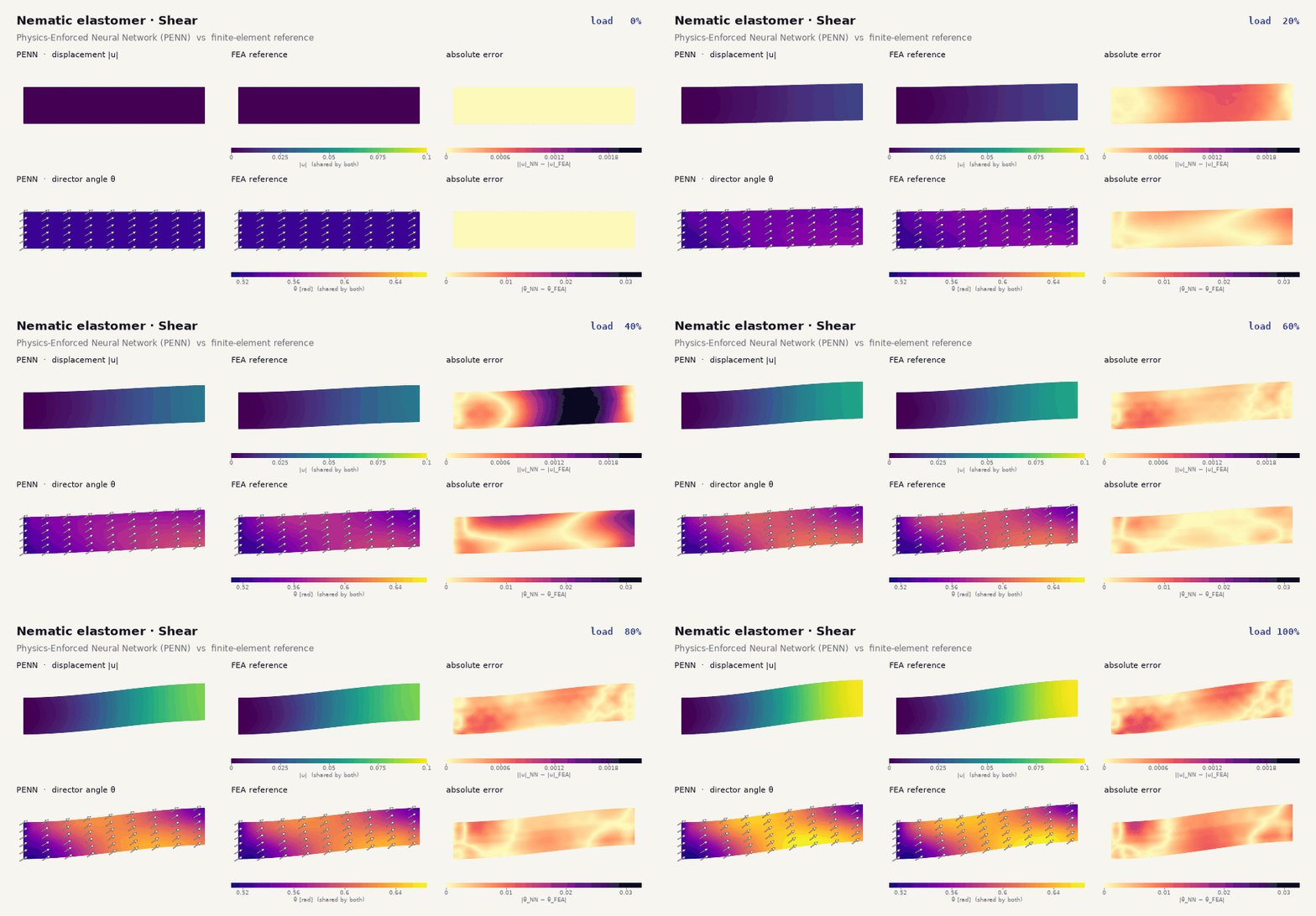
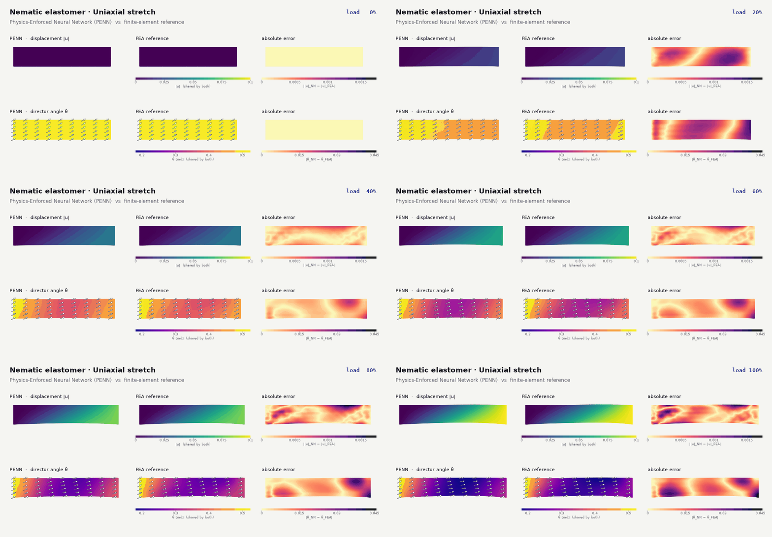
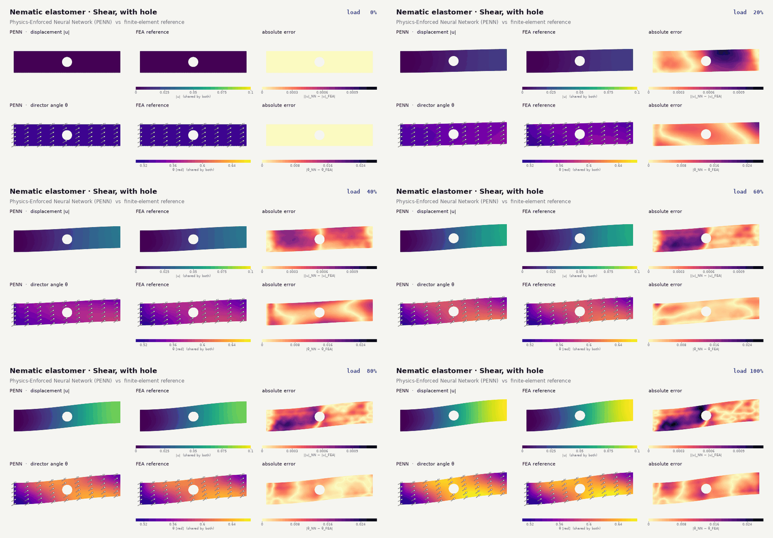
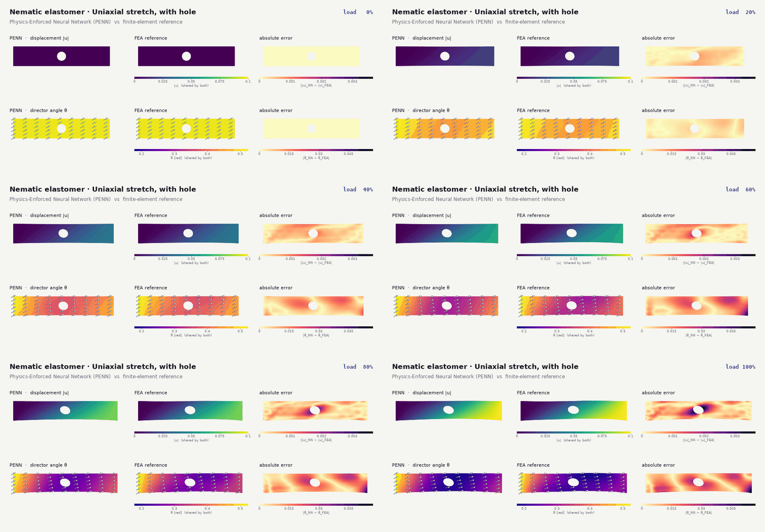
The problem is solved on a thin strip with four loading cases: shear and uniaxial stretch, each with and without a circular hole. The Physics-Enforced Neural Network (PENN) and the DeepONet are each compared with a finite-element (FEA) reference.

Physics-Enforced Neural Network (PENN)

A Physics-Enforced Neural Network represents the deformation and the director field with separate networks, builds the unit-length constraint on the director into the architecture, and is trained by minimizing the total potential energy of the system, with no solution data. Each animation shows the load ramp, with the network prediction, the finite-element reference and the pointwise error side by side: displacement magnitude on top, director angle below.

Operator learning: DeepONet

A DeepONet learns an operator, not a single solution. In the standard construction, a branch network encodes the input, here the load level, and a trunk network encodes the position in the body, and their combination gives the deformation and director fields at that position. After training, any load on the ramp is evaluated with one forward pass, so a single model covers the whole load ramp. The same four cases are shown below, with the DeepONet prediction, the finite-element reference and the pointwise error.

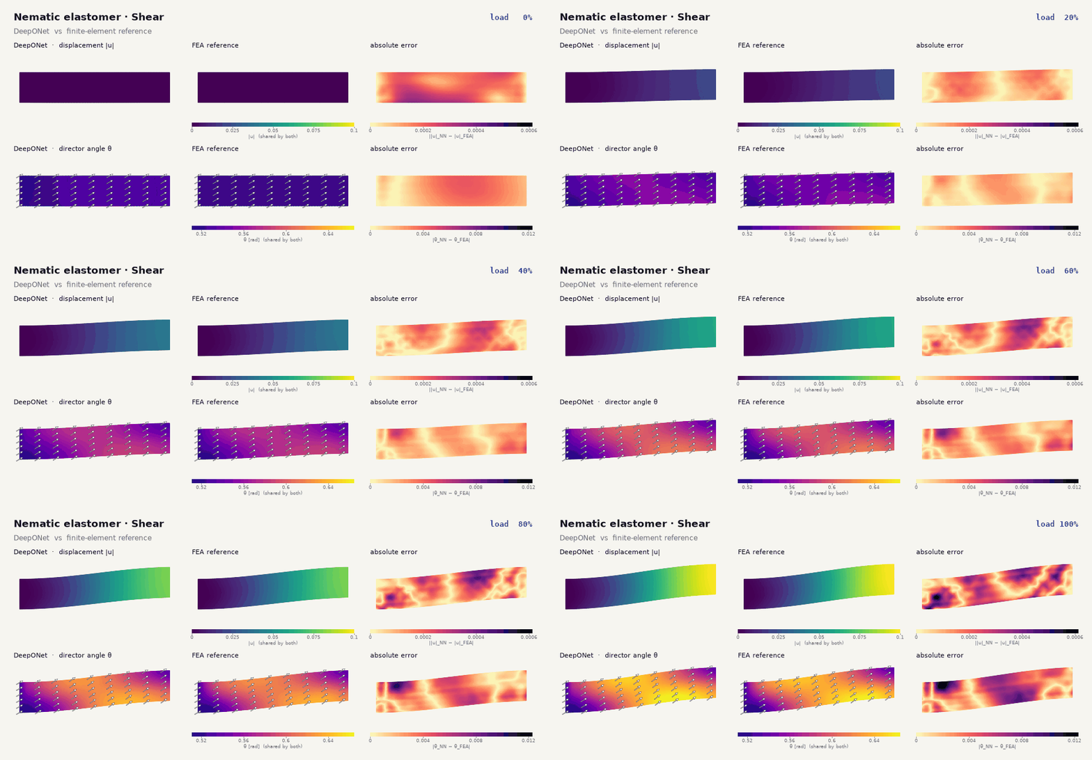
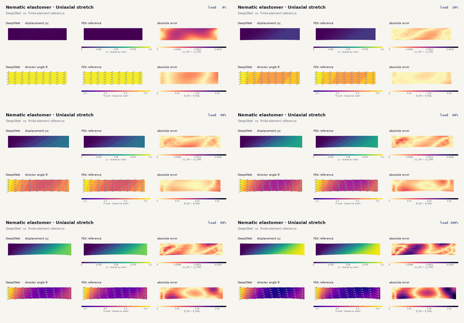
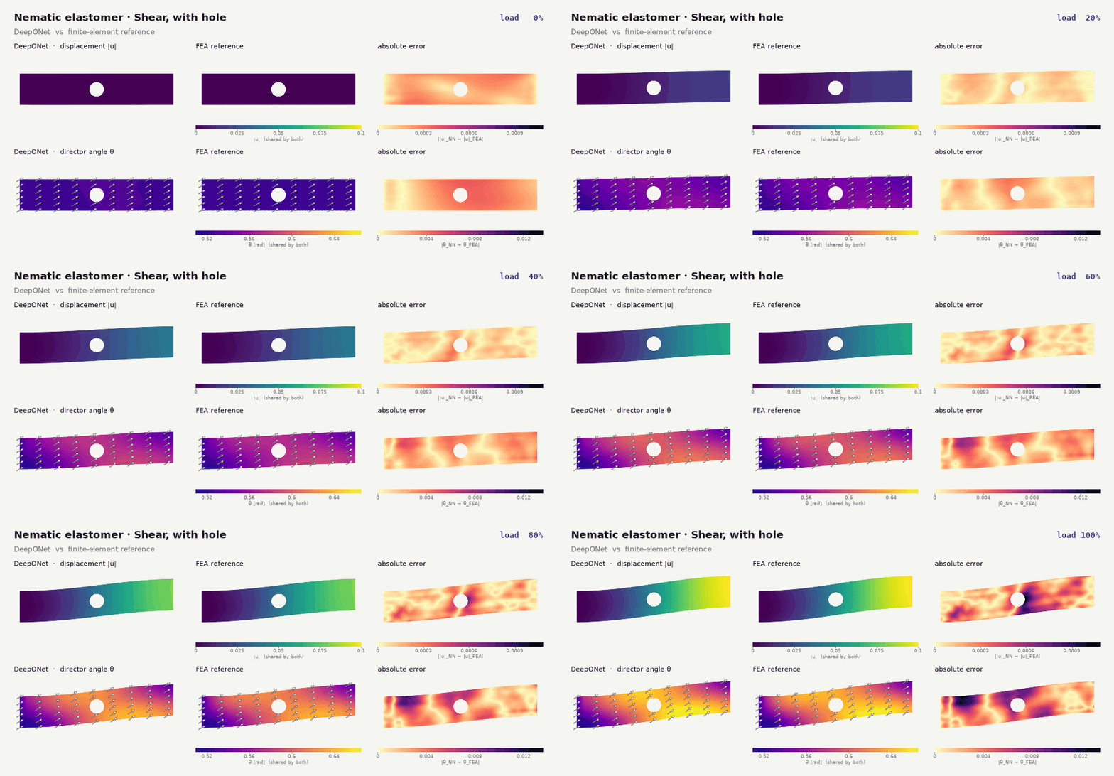
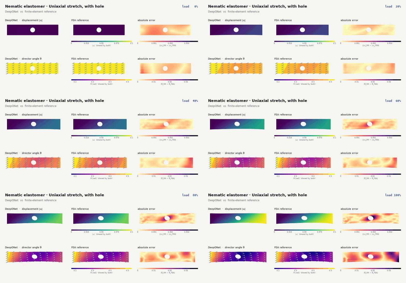
Animations are interpolated between the stored load steps for smooth playback. The reference in every panel is a finite-element solution of the same discretized problem. Work in progress.

Validating network output: three necessary conditions

Satisfying the balance laws is not enough: a stationary point can be a saddle or a maximum. At a stable equilibrium \( (\boldsymbol{\chi}_e,\boldsymbol{d}_e) \) the energy cannot be lowered by any admissible perturbation,

Choosing localized perturbations (a compactly supported displacement \( \boldsymbol{\Phi} \) and a director rotation built from an axial field \( \boldsymbol{w} \)) and shrinking their support to a point yields a hierarchy of conditions. They are necessary for any energy minimizer, whether it comes from finite elements, a neural network or an analytical solution, so a state that violates one cannot be a stable minimizer and can be rejected.

The three are ordered by strength: polyconvexity \( \Rightarrow \) quasiconvexity \( \Rightarrow \) rank-one convexity \( \Rightarrow \) Legendre–Hadamard. They are necessary, not sufficient: passing them does not prove a state is the global minimizer, but failing any one disqualifies it.

Applied to this model

For the energy above and unit vectors \( \boldsymbol{s} \) and \( \boldsymbol{T} \), the deformation modulus is

where \( \cos\lambda=\boldsymbol{s}\cdot\boldsymbol{d} \) and \( \cos\lambda_{0}=\boldsymbol{T}\cdot\boldsymbol{D} \). For the shape anisotropy \( r=2 \) used here this becomes

so the strong ellipticity condition, the strong form of the Legendre–Hadamard inequality,

is satisfied, and the chosen constitutive model and parameter set are strongly elliptic within the regime considered. Two consequences for validation:

• For this energy, Legendre–Hadamard holds a priori. Checking it on network output confirms that the output is an admissible state, but it cannot expose a poor solution by itself.
• The conditions become discriminating for energies that are not elliptic by construction, such as learned or data-driven constitutive models, and for the global quantities below.

What is checked on the computed solutions

For every stored trajectory (finite element, PENN and DeepONet), two computational checks are applied to the nodal solutions:

• Strong ellipticity at every Gauss point: the smallest eigenvalue of the acoustic tensor built from the deformation modulus \( \mathscr{M} \), scanned over all in-plane directions \( \boldsymbol{T} \), with the director held at its local value.
• Second variation at every load step: the smallest eigenvalue of the reduced Hessian of the discretized total energy with respect to the free displacement and director degrees of freedom. A positive value means a strict local minimizer of the discrete problem rather than a saddle.

All stored trajectories pass both checks: positive acoustic-tensor eigenvalue at every Gauss point and no negative Hessian eigenvalues. A passing check means the states are consistent with these necessary conditions and are strict local minimizers of the discretized energy. It does not mean the networks match the finite-element solution; that is what the animations above show, and both the PENN and the DeepONet remain visibly less accurate than FEA, especially in director angle. The Legendre–Hadamard check implemented here covers the deformation block with the director held fixed; the fully coupled form above is satisfied analytically for this model but is not separately evaluated numerically.

Reference

[1] M. Shirani, P. H. Gueldner, M. Khidoyatov, J. L. Warren, F. Ninno, Physics-Consistent Neural Networks for Learning Deformation and Director Fields in Microstructured Media with Loss-Based Validation Criteria, arXiv:2603.06939 (2026). arxiv.org/abs/2603.06939 ↗